SymCode: The Symbolic Barcode for Humans and Machines
Researchers: Chris Tsang and Sanford Pun | Published: 2021-04-03
This is our story of the design and implementation of a symbolic barcode system. Try the Demo Web App on symcode.visioncortex.org.
Forewords
If you are lucky enough to live in a place where an Amazon Go store is nearby, you definitely should visit it. It is packed full of esoteric technology that enthusiast like us get super intrigued. One item that caught our eyes was the labels on the salad and sandwiches in the ready-made food section.
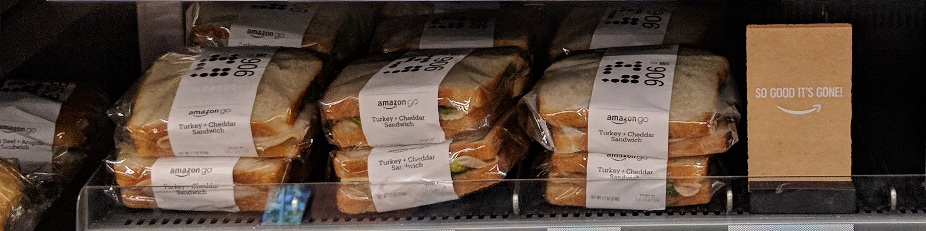
Photo within an Amazon Go store
Photo by Sikander Iqbal via Wikimedia Commons
.jpg)
There printed a matrix of cute little circles and squares! It must be a barcode of some sort. Our attempt to decipher the 'Amazon Reversi Code' was futile, but this is the start of the story.
Background
A bit of context for the unfamiliar reader, the name Barcode is referring to the labels we still find in virtually every packaged products today. Barcode encode data by varying the widths and spacings of the vertical bars, which are to be scanned by a laser beam crossing horizontally. With the advent of image sensors, 2D barcodes were developed, where QR code and Aztec Code are some of the most well-known.
In general, 2D barcode scanner works as follows:
Locate the finders. These finders act as a trigger to tell the scanner that 'here is a barcode!'. The finders have to be easily detectable yet not interfering with the data modules.
Attempt to scan and read metadata surrounding the finder candidates. The metadata usually includes a format code and timing patterns.
If the previous step succeeds, the scanner would sample the entire barcode to construct a raw bit string. A checksum operation is done to detect errors.
If the previous step succeeds, the payload is extract from the raw bits, which usually involves some bit masking and shuffling.
This framework has aged well and they are quite robust and low-cost to implement in embedded systems. However, they are meant to be read by machines and not by our naked eyes. They are not designed for aesthetics and are impossible for humans to comprehend.
Goals and Constraints
Our goal is to design a barcode system that are both human-readable and machine-readable. We now turn our attention to human readability by studying human languages.
Machines run on bits, so we can say the alphabet consists of 0 and 1. In human languages, we have a larger set of alphabets. In English, we have 26 distinct lowercase letters. In Korean, characters are constructed by composing 2 to 6 elements from a set of 40 distinct Jamo.
There is a direct tradeoff between information density and visual ambiguity. If the symbol set is too large, humans would have difficulty in remembering all of them. In addition, there may be some visually similar symbols that are hard to disambiguate. If the symbol set is too small, the same message has to be encoded with more symbols, which again, humans often have a hard time in processing long strings.
We determined that a symbol set in the range of 16 to 64 symbols is a good balance.
Design of symbols
What makes good symbols?
Prominence
First, the symbols have to stand out from the natural world, to manifest that they are created deliberately to convey a message but not a result of some natural phenomenon.
Repeatable
Symbols are constructed with specific tools and processes that can be taught to other people. The meaning of a symbol should remain the same when reproduced, in which variation is tolerated.
Distinctive
Symbols within a set should not be similar with each other and have distinctive features allowing the reader to resolve ambiguity between symbols.
Aesthetics
Finally, good symbols should observe the aesthetics rules of the human eye, including being anti-symmetric, rotational symmetric, balanced and consistent. As a pointer, the Gestalt Principles are fantastic rules of thumb.
With the above rules in mind, we designed a minimalistic symbol set. Each symbol is composed of multiple triangles, the basic geometric primitive. Each symbol is symmetric or anti-symmetric in overall, but exhibits asymmetry internally. They are like Tangram, in which a human child can easily reproduce the symbols by assembly some triangular pieces together.
The next section would quantitatively analyze and justify this design methodology.
Trace of shapes
The naive way to match a shape against a symbol set is to perform a linear search, XOR it with every symbol and then chooses the one with the lowest delta. It works in principle, but is inefficient. Ideally, an algorithm can condense a complex shape into a feature vector, which we can lookup in the feature space of the symbol set for the nearest neighbour and arrive to a match.
Instead of using an array of real numbers, we devised that an array of bits are sufficient to capture the essence of symbols, and from now on we refer this bit string as 'trace'.
The English alphabet
Now, let us take a closer look at the lowercase English alphabet set to illustrate this idea.

English alphabets
First off, we can classify the 26 alphabets as either tall or short, giving:
Tall: b d f g h j k l p q t yShort: a c e i m n o r s u v w x z
Next, we can divide the letter into two halfs horizontally and compare their weights:
Left > right: b c f h k p r t yLeft < right: a d g qLeft ~ right: e i j l m n o s u v w x z
Then, we can divide the letter into two halfs vertically and compare their weights:
Up > down: f m n p q r yUp < down: b d h k uUp ~ down: a c e g i j l o s t v w x z
At this point, we had the following:
a: SR=b: TLDc: SL=d: TRDe: S==f: TLUg: TR=h: TLDi: S==j: T==k: TLDl: T==m: S=Un: S=Uo: S==p: TLUq: TRUr: SLUs: S==t: TLDu: S=Dv: S==w: S==x: S==y: TLUz: S==
Group by trace:
SR=: aTLD: b h kSL=: cTRD: dS==: e i o s v w x zTL=: tTR=: gT==: j lS=U: m nTLU: f p yTRU: qSLU: rS=D: u
Which is a surprisingly good classifier using only three comparisons. We can do more trinary comparisons on smaller partitions to further differentiate the collisions, but our investigation on English alphabets ends here for the scope of this article.
SymCode
Our trace for SymCode symbols follows a similar scheme. We define the symbol traces starting from the three comparisons defined in the previous section.
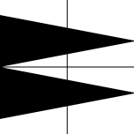
The pixel count in each of the four quadrants of a symbol (in order of top-left, top-right, bottom-left, bottom-right) are denoted by non-negative quantities a,b,c,d respectively, the three comparisons are defined as follows:

Grid quadrants
- Vertical comparison =
(a+b)vs(c+d) - Horizontal comparison =
(a+c)vs(b+d) - Diagonal comparison =
(a+d)vs(b+c)
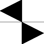
Below are two examples:
LongRR symbol image
- Vertical comparison = Top ~ Bottom
- Horizontal comparison = Left > Right
- Diagonal comparison = Backslash ~ Slash
SmallDoubleLR symbol image
- Vertical comparison = Top ~ Bottom
- Horizontal comparison = Left ~ Right
- Diagonal comparison = Backslash > Slash
Each comparison has 3 possible outcomes (<, >, ~). For simplicity, we assign 2 bits to encode each comparison. Therefore, this naive implementation uses 3 * 2 = 6 bits to store each trace.
The above worked well enough for sets of 16 symbols, but it was found inadequate for 32 symbols. Acute32 requires more comparisons for traces.
Trace of SymCode
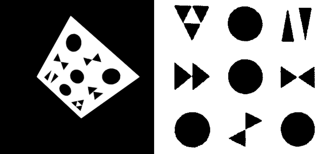
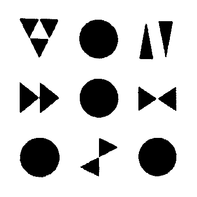
The following figure is Acute32's alphabet set.
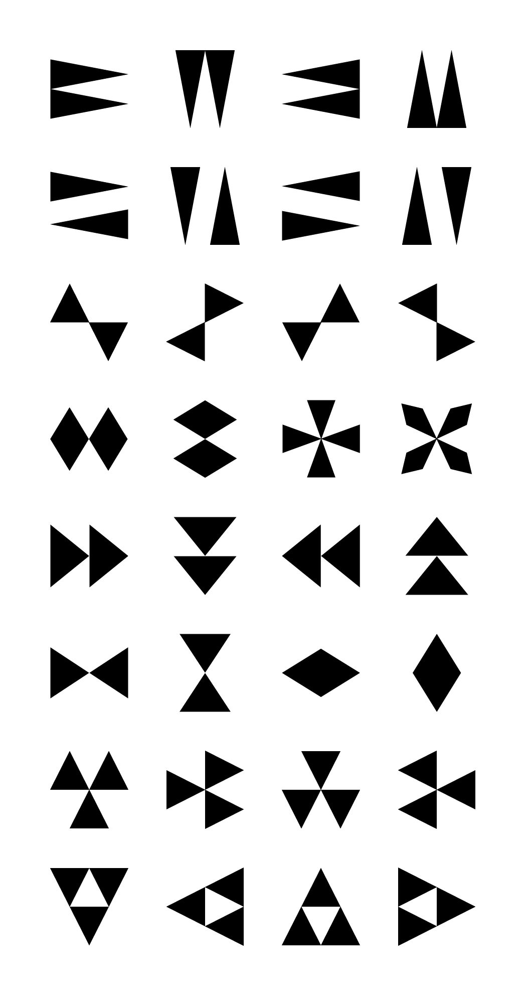
Acute32 alphabet set
Apart from the three basic comparisons explained in the previous section (V,H,D), we also compare every pair of the four quadrants (each quadrant is compared to every other quadrant exactly once), requiring an extra of 4 choose 2 = 6 comparisons (ab, cd, ac, ...). The last comparison efgh is explained in the details below.
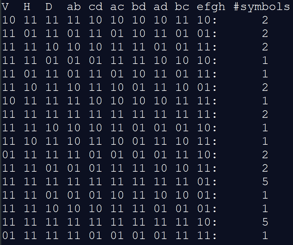
Acute32 trace counts
Side note: efgh
It is important to note that not any arbitrary extra comparisons are effective. The rule of thumb is each extra comparison should introduce new information than the existing ones, making them (at least partially) independent of each other. In general, comparisons that use different numbers of blocks should be independent. For example, in the previous section all comparisons used 2 blocks vs 2 blocks, so the extra ones in this section, which use 1 block vs 1 block, are all (partially) independent of the previous ones. This is because as more blocks are being considered at once, the scope of analysis becomes irreversibly broader - just like how you cannot retrieve neither x nor y from the sum x+y.
Adding the extra ones results in a total of 3 + 6 = 9 comparisons. Using 2 bits to encode each, we are using 9 * 2 = 18 bits to store each trace in Acute32.
Denote a comparison operation by "U vs V". The vertical, horizontal, and diagonal comparisons become "Top vs Bottom", "Left vs Right", and "Backslash vs Slash" respectively. The rest of the comparisons become "a vs b", "c vs d", and so on. We set the bits as follows:
For each comparison U vs V
- 11 means "U ~ V"
- 10 means "U > V"
- 01 means "U < V"
- 00 is invalid
The trace of all 1's, which happens when all four quadrants of the symbol share (approximately) the same number of dots, is shared by about one-third of the entire Acute32. This makes approximately one-third of the searches scan through 12 symbol images, which is 4 times that of most of the rest, which only scan through 3 symbol images.
Our solution here is one more comparison.
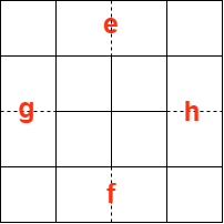
efgh (top/bottom/left/right) grid
We further partition the grid of each symbol image so that there are 4x4 = 16 small blocks, and denote the top/bottom/left/right blocks along the edge by e,f,g,h respectively, as illustrated in the figure above. Next, we define an "ef/gh comparison" which compares e+f to g+h.
Now we have a more balanced distribution.
Advantages of traces
The trace partitions the symbol set into smaller, mutually-exclusive subsets. This enhances robustness against noisy inputs.
As searching through traces is much more efficient than comparing with each symbol individually, traces also help with performance.
Most importantly, it provides us a guidance in designing the symbols to maximize differences within the symbol set.
Scanning Pipeline
The pipeline of SymCode scanner consists of 4 stages: finder, fitter, recognizer, decoder.
Each stage below begins with a more general description of the processing stage (general across any SymCode), followed by explanation of the implementation of Acute32.
Stage 1: Locating Finder Candidates
We first binarize the input color image using an adaptive thresholding strategy, shapes are then extracted from a binary image by clustering.
The goal of this stage is to find the positions of all finder candidates in the frame.
A minimum of 4 feature points is needed because at least 4 point correspondences are required to fit a perspective transform.
Acute32
Acute32 uses circles as finders because they are distinct from the heavily cornered symbol set. The 4 finders are arranged in a Y shaped manner to break the rotational symmetry with itself.
The advantage of using a circle is that, in general, it always transforms into an ellipse under any perspective distortion, making it relatively easy to detect.
The disadvantage is the lack of corners in circles. It is too easy to detect false positives because there are indeed many circles in real life.
Stage 2: Fitting Perspective Transform
We define the "image space" as the space of pixels on the input frame, and the "object space" as the space of pixels on the code image (whose boundary is predefined). An image space is simply the input frame image. An object space can either be generated using a code instance, or by rectifying the corresponding image space.
Left: image space; Right: object space
In essence, this stage chooses the correct perspective transform to be used in the next stage.
Each perspective transform converts the image space into an object space (but not necessarily the correct one) and is defined by (at least) 4 point pairs (source and destination points), where each pair consists of a point in the image space and the other one in the object space.
Since we have obtained a list of finder candidates from the previous stage, we can extract n feature points in the image space from them. Matching the 4-permutations of them to the 4 predefined feature points in the object space gives us at most n permute 4 = k perspective transforms.
It is inefficient to accept each transformation and generate k object spaces to proceed to next stage. Therefore, we need to design a method to evaluate each transform and chooses which ones to proceed. The simplest way is to define some extra feature points in the object space as check points, which are re-projected to the image space, and check if the feature exists there, and reject the candidate otherwise.
Acute32
The re-projection method mentioned above could not work for us because circles do not provide extra feature points for us to verify.
Instead, we take each of the k perspective transforms and calculates an error value.
We define 4 object check points as the top of the 4 circle finders in the object space. Re-projecting these 4 points to the image space, we obtain the image check points (i1 to i4). Furthermore, we denote the centres of the circle finders in the image space, in the same order as the previously defined points, by c1 to c4.
Our metric of evaluation relies on magnitude and direction of the difference vector. 4 vectors interest us here: the vectors from the centres of finders to the image check points, and we denote them by v1 to v4 respectively.
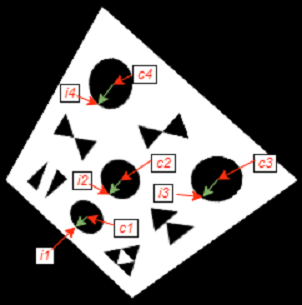
Transform evaluation points and vectors: the 4 green vectors are v1 to v4
We observed that given a correct transform, the 4 green vectors are consistently pointing in the same direction, with their magnitudes less uniform but still very similar. We found it effective to choose the transform with the minimum variance among v1 to v4.
Stage 3: Recognizing Symbols
In the previous stage, we have obtained a perspective transform which converts between the image and object spaces. Next, we're going to rectify the input image into a code image, and recognize the symbols on it.
Rectify the image space
Once we have a transform that we believe is correct, the object space can be obtained by applying it on the image space. We sample the image with bilinear interpolation.
Recognition
Rectified image (code image in the correct object space)
Assuming the transform is correct, the coordinates of the symbols on the code image should be close to the anchors we defined in the object space.
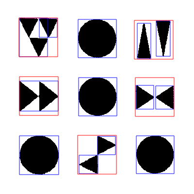
Recognition process marked by bounding boxes
The bounding boxes in blue are all clusters found on the code image. The boxes in red are the grouped clusters used to recognize each symbol.
Once we have the images, we can evaluate their traces and compare them with the ones in our symbol library, obtaining a small number of candidates for each symbol image. Each of these candidates is compared to the symbol image and the one with the lowest delta is the final recognized symbol.
Each symbol is mapped to a unique bit string, and they are concatenated into a longer bit string.
Stage 4: Decoding the SymCode
This stage performs error detection (possibly correction) and extract the payload.
Acute32
As there are 32 symbols in the set of Acute32, each symbol can encode 5 bits. There are 5 data symbols and 4 finders in the 3x3 configuration. It can easily be extended to a 6x4 to carry more data. For now, each SymCode instance encodes 25 raw bits, where 20 bits are payload and 5 bits are CRC checksum.
Conclusion
We developed a theoretic as well as a programming framework for designing and implementing symbolic barcodes. The programming library is available as symcode. For those who simply want to integrate SymCode into your application, please refer to the wasm distribution acute32 which is ready to use in any browser based Javascript projects.
About Vision Cortex
This story is a manifest of the philosophy behind Vision Cortex, and a glimpse of the ongoing research and development by the Vision Cortex Research Group.
If you enjoyed the reading and appreciate our work, consider starring (on GitHub), discuss (on Reddit / GitHub), share (on Twitter) and collaborate.